Random matrix theory and $\zeta(s)$
number-theory asymptotics algebraIn 1973, Montgomery conjectured that, assuming the Riemann hypothesis, the number of pairs of zeros ${1\over2}+i\gamma$ and ${1\over2}+i\gamma'$ of $\zeta(s)$ satisfying
\[{\gamma-\gamma'\over2\pi}\log T\in[\alpha,\beta], \qquad \gamma,\gamma'\in[0,T],\]is asymptotic, as $T\to+\infty$, to
\[{T\over2\pi}\log T \left\{ \int_\alpha^\beta \left[1-\left({\sin\pi u\over\pi u}\right)^2\right]\mathrm d u +\mathbf 1_{0\in[\alpha,\beta]} \right\}.\]Dyson observed that the density inside this formula is the two-level correlation density of eigenvalues of large random unitary matrices. This connection gives a model not only for the spacings between zeros of $\zeta(s)$, but also for the distribution of its values on the critical line $\operatorname{Re}(s)={1\over2}$.
This post surveys the random matrix model for the Riemann zeta function, from Montgomery's pair correlation conjecture to the Keating–Snaith conjecture for the moments
\[I_k(T)={1\over T}\int_0^T \left\vert\zeta\left({1\over2}+it\right)\right\vert^{2k}\mathrm d t.\]The epilogue gives one glimpse of how the model extends beyond $\zeta(s)$. A more technical account of the material in this post is available in the accompanying PDF.
Montgomery's conjecture
The Riemann zeta function is initially defined by
\[\zeta(s)=\sum_{n=1}^\infty{1\over n^s}=\prod_p(1-p^{-s})^{-1},\qquad \operatorname{Re}(s)>1.\]Its analytic continuation has nontrivial zeros in the critical strip $0<\operatorname{Re}(s)<1$. The Riemann hypothesis predicts that all of them have the form
\[\rho={1\over2}+i\gamma.\]Let $N(T)$ count the ordinates $0<\gamma\le T$. The Riemann–von Mangoldt formula implies
\[N(T)\sim{T\over2\pi}\log T,\]so the mean gap near height $T$ is about ${2\pi\over\log T}$. To compare gaps at different heights, we therefore normalize a difference $\gamma-\gamma'$ by considering
\[{\gamma-\gamma'\over2\pi}\log T.\]The question is no longer where each zero lies, but how often two normalized zeros are a given distance apart.
Pair correlation of zeros
By pair correlation, we mean the measure obtained by counting ordered pairs $(\gamma,\gamma')$ of zero ordinates up to height $T$ whose normalized difference lies in a given interval, and dividing by $N(T)$.
Assuming the Riemann hypothesis, Montgomery (1973)1 studied the pair correlation of zeta zeros and was led to the following conjectural density:
\[1-\left({\sin\pi u\over\pi u}\right)^2.\]More precisely, after excluding the diagonal pairs $\gamma=\gamma'$, the normalized differences should satisfy
\[{1\over N(T)}\#\left\{\gamma,\gamma'\in(0,T],\ \gamma\ne\gamma': {\gamma-\gamma'\over2\pi}\log T\in[\alpha,\beta]\right\} \longrightarrow \int_\alpha^\beta\left[1-\left({\sin\pi u\over\pi u}\right)^2\right]\mathrm d u.\]Near $u=0$ this density vanishes quadratically. Thus nearby zeros repel one another: very small gaps occur less often than they would in a collection of independent random points.
The remarkable step came when Freeman Dyson recognized this density. It was already known as the two-point correlation density for eigenvalues of large random unitary matrices.
The circular unitary ensemble
The unitary group is
\[U(N)=\{A\in\mathbb C^{N\times N}:A^\ast A=I\}.\]It is a compact group, so it carries a unique translation-invariant probability measure, called Haar measure and denoted by $\mu_{\mathrm{CUE}}$. This is the matrix analogue of uniform measure: multiplying every matrix by a fixed unitary matrix does not change the distribution. The probability space $(U(N),\mu_{\mathrm{CUE}})$ is called the circular unitary ensemble (CUE).
Distribution of eigenvalues
Every $A\in U(N)$ has eigenvalues on the unit circle. Write them as
\[e^{i\theta_1},e^{i\theta_2},\ldots,e^{i\theta_N},\qquad 0\le\theta_j<2\pi.\]Set
\[E=\operatorname{diag}(e^{i\theta_1},\ldots,e^{i\theta_N}).\]A continuous class function $h$ on $U(N)$ is constant under conjugation, so it depends only on the unordered eigenvalues of $A$. Conversely, every continuous symmetric function of the eigenvalues defines a class function. Thus the joint eigenvalue distribution is determined by the integrals
\[\int_{U(N)}h(A)\mathrm d\mu_{\mathrm{CUE}}(A)\]for all continuous class functions $h$. The Weyl integration formula evaluates these integrals in eigen-angle coordinates:
\[\begin{aligned} \int_{U(N)}h(A)\mathrm d\mu_{\mathrm{CUE}}(A) &={1\over(2\pi)^N N!} \int_{[0,2\pi)^N}h(E)\\ &\qquad\times \prod_{1\le j<\ell\le N} \vert e^{i\theta_j}-e^{i\theta_\ell}\vert^2 \mathrm d \theta_1\cdots\mathrm d \theta_N. \end{aligned}\tag{1}\]Formula (1) therefore identifies the joint density of the eigen-angles as
\[P_N(\theta_1,\ldots,\theta_N) ={1\over(2\pi)^N N!} \prod_{1\le j<\ell\le N}\vert e^{i\theta_j}-e^{i\theta_\ell}\vert^2.\]It vanishes whenever two eigen-angles coincide, making eigenvalue repulsion visible directly in the probability law.
Correlation of eigenvalues
The squared Vandermonde factor does more than determine the density: it makes the CUE eigen-angles a determinantal point process. If $R_{N,n}(\theta_1,\ldots,\theta_n)$ denotes the density for ordered choices of $n$ distinct eigen-angles, then it is obtained from the joint density by
\[R_{N,n}(\theta_1,\ldots,\theta_n) ={N!\over(N-n)!} \int_{[0,2\pi]^{N-n}}P_N(\theta_1,\ldots,\theta_N) \mathrm d \theta_{n+1}\cdots\mathrm d \theta_N.\tag{2}\]To evaluate (2), one expands the Vandermonde determinant and its conjugate, uses orthogonality to integrate out $\theta_{n+1},\ldots,\theta_N$, and recognizes the remaining sum of squared minors by Gram's identity. The result is
\[R_{N,n}(\theta_1,\ldots,\theta_n) =\det(K_N(\theta_j,\theta_\ell))_{j,\ell},\]where
\[K_N(\alpha,\beta)={1\over2\pi} {\sin {N\over2}(\alpha-\beta)\over \sin {1\over2}(\alpha-\beta)}.\]Thus every finite-level correlation is controlled by one kernel. The mean spacing of $N$ points around a circle of length $2\pi$ is ${2\pi\over N}$. Hence the normalized $n$-level correlation density is
\[\left({2\pi\over N}\right)^n R_{N,n}\left({2\pi x_1\over N},\ldots,{2\pi x_n\over N}\right) =\det\left({1\over N}{\sin\pi(x_j-x_\ell) \over\sin {\pi\over N}(x_j-x_\ell)}\right)_{1\le j,\ell\le n}.\]For $j\ne\ell$, the denominator satisfies $N\sin({\pi\over N}(x_j-x_\ell))\to\pi(x_j-x_\ell)$, while the diagonal entries are identically $1$. Since $n$ is fixed and the determinant is a polynomial in its entries, we may pass to the limit entry by entry. This gives the scaling limit
\[W_n(x_1,\ldots,x_n)= \det\left({\sin\pi(x_j-x_\ell) \over\pi(x_j-x_\ell)}\right)_{1\le j,\ell\le n}.\tag{3}\]In particular, when $n=2$,
\[W_2(x,y)=1-\left({\sin\pi(x-y)\over\pi(x-y)}\right)^2,\]exactly the expression in Montgomery's conjecture. Matching
\[{2\pi\over N}\approx{2\pi\over\log T}\]suggests that zeros near height $T$ should be compared with eigenvalues of matrices of size $N\approx\log T$. This comparison does not explain the locations of individual zeros. It predicts that, at the scale of the mean spacing, all their local correlation statistics are governed by the same limiting process as CUE eigenvalues.
Values of $\zeta(s)$ on $\operatorname{Re}(s)={1\over2}$
The correspondence between zeta functions and random matrices extends beyond zeros and eigenvalues. We now turn from local spacing statistics to the distribution of values on the critical line.
Selberg's central limit theorem
Selberg's central limit theorem says that, for typical $t$ near $T$,
\[\log\left\vert\zeta\left({1\over2}+it\right)\right\vert\]is approximately normal with mean $0$ and variance ${1\over2}\log\log T$. Selberg's theorem describes the bulk distribution of $\log\vert\zeta({1\over2}+it)\vert$, but says little about its large deviations.
Moments of $\vert\zeta({1\over2}+it)\vert$
One way to investigate these exceptional values is through the moments
\[I_k(T)={1\over T}\int_0^T\left\vert\zeta\left({1\over2}+it\right)\right\vert^{2k}\mathrm d t.\]A naive Gaussian extrapolation predicts $I_k(T)\sim(\log T)^{k^2}$ but not the correct leading constant. Hardy–Littlewood (1918)2 proved
\[I_1(T)\sim\log T,\]while Ingham (1926)3 proved
\[I_2(T)\sim{1\over2\pi^2}(\log T)^4.\]The exponent $k^2$ is correct in both cases, but the fourth moment already shows that a Gaussian model alone cannot determine the coefficient.
The arithmetic part of that coefficient can be motivated by a Dirichlet polynomial approximation. For $k>0$, write $\tau_k(n)$ for the coefficients of $\zeta(s)^k$. For a suitable length $X$, the heuristic models $\zeta({1\over2}+it)^k$ by
\[\sum_{n\le X}{\tau_k(n)\over n^{1/2+it}}.\]The approximate orthogonality of $n^{-it}$ over $t\in[0,T]$ then suggests that the main term of $I_k(T)$ should be related to
\[\sum_{n\le X}{\tau_k(n)^2\over n} \sim {a_k\over\Gamma(k^2+1)}(\log X)^{k^2}.\]Here the Euler product gives
\[a_k=\prod_p\left(1-{1\over p}\right)^{k^2} \left(1+\sum_{r=1}^\infty{\tau_k(p^r)^2\over p^r}\right).\]This is the arithmetic factor. The remaining universal factor is predicted by characteristic polynomials of random unitary matrices.
Characteristic polynomials in CUE
For $A\in U(N)$, define its characteristic polynomial on the unit circle by
\[Z(A,\theta)=\det(I-Ae^{-i\theta}).\]It vanishes precisely when $e^{i\theta}$ is an eigenvalue of $A$. This makes $Z(A,\theta)$ a finite-dimensional counterpart of $\zeta(s)$: both are analytic objects built from a spectrum of zeros. In terms of the eigen-angles,
\[Z(A,\theta)=\prod_{j=1}^N(1-e^{i(\theta_j-\theta)}).\]The product above is the finite-dimensional analogue of the Hadamard product for $\zeta(s)$. Taking absolute values and logarithms turns both products into sums over their zeros. Haar invariance under $A\mapsto Ae^{-i\theta}$ also means that the distribution of $Z(A,\theta)$ does not depend on the chosen angle $\theta$.
On the random matrix side, $\log\vert Z(A,\theta)\vert$ is approximately normal with variance ${1\over2}\log N$. The identification $N\approx\log T$ therefore matches Selberg's central limit theorem.
The analogy is visible even before taking an asymptotic limit. After scaling all three distributions to unit variance, Keating–Snaith (2000)4 compared $\operatorname{Re}\log Z$ for CUE with $N=42$, $\operatorname{Re}\log\zeta({1\over2}+it)$ near the $10^{20}$-th zero, and a standard Gaussian. The CUE and zeta curves nearly coincide, while the Gaussian remains visibly different.
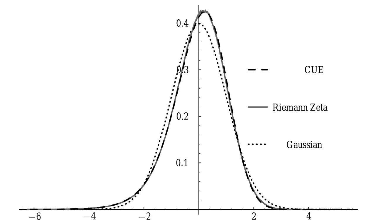
Soundararajan captured the striking contrast in his 2022 ICM plenary lecture5:
There is so much support for a conjecture which goes beyond the Riemann hypothesis and so little support for a theorem, at least numerically.
The comparison also extends from the bulk distribution to moments. For real $k>-{1\over2}$, the corresponding CUE moment can be evaluated exactly:
\[\int_{U(N)}\vert\det(I-A)\vert^{2k}\mathrm d\mu_{\mathrm{CUE}}(A) =\prod_{j=1}^N{\Gamma(j)\Gamma(j+2k)\over\Gamma(j+k)^2}.\]As $N\to\infty$, this is
\[\sim {G(1+k)^2\over G(1+2k)}N^{k^2},\]where $G$ is the Barnes $G$-function. This asymptotic supplies the universal factor. Since primes do not enter the random matrix model, however, the CUE calculation alone cannot produce the entire leading constant for $I_k(T)$.
Combining this universal factor with the arithmetic factor $a_k$ gives the Keating–Snaith conjecture:
\[I_k(T)\sim {g_ka_k\over\Gamma(k^2+1)}(\log T)^{k^2},\tag{4}\]where
\[g_k=\Gamma(k^2+1){G(1+k)^2\over G(1+2k)}.\]For $k=1$ this recovers the classical second moment, and for $k=2$ it recovers Ingham's fourth moment.
Hybrid model
To place the random matrix and arithmetic components in one framework, Gonek–Hughes–Keating (2007)6 developed a hybrid Euler–Hadamard model. Assuming RH, a schematic local form near $s={1\over2}+it$ is
\[\zeta(s)\approx \prod_{p\le X}(1-p^{-s})^{-1}\times \prod_{\substack{\rho_n={1\over2}+i\gamma_n\\ \vert t-\gamma_n\vert\le {1\over\log X}}} \left[(s-\rho_n)e^\gamma\log X\right],\]where $\gamma=0.5772\ldots$ is Euler's constant. The first product is the Euler component $P_X$, and the second product is the Hadamard component $Z_X$.
The splitting conjecture treats the two components as asymptotically independent:
\[I_k(T)\sim {1\over T}\int_0^T\vert P_X\vert^{2k}\mathrm d t \cdot {1\over T}\int_0^T\vert Z_X\vert^{2k}\mathrm d t.\]The Euler component has the asymptotic
\[{1\over T}\int_0^T\vert P_X\vert^{2k}\mathrm d t \sim a_k(e^\gamma\log X)^{k^2},\tag{5}\]while the characteristic-polynomial model predicts
\[{1\over T}\int_0^T\vert Z_X\vert^{2k}\mathrm d t \sim {G(1+k)^2\over G(1+2k)} \left({\log T\over e^\gamma\log X}\right)^{k^2}.\tag{6}\]Multiplying (5) and (6) cancels the powers of $e^\gamma\log X$ and recovers the Keating–Snaith conjecture (4).
Progress towards moments
Full asymptotic formulas for $I_k(T)$ are known only for $k=1$ and $k=2$. For broader ranges of $k$, the known lower bounds have the conjectural magnitude
\[I_k(T)\ge c_k(\log T)^{k^2},\tag{7}\]for every real $k>0$. Progress toward (7) took several steps. Ramachandra (1978, 1980)7 proved it for positive half-integers $k$, and Heath-Brown (1981)8 extended it to positive rational $k$. Radziwill–Soundararajan (2013)9 obtained it for every real $k\ge1$, with the explicit choice $c_k=e^{-30k^4}$. Heap–Soundararajan (2020)10 then treated $0<k\le1$, completing the lower-bound picture for all positive real $k$.
The corresponding conjectural upper bound is
\[I_k(T)\ll_k(\log T)^{k^2}.\tag{8}\]The history of (8) is subtler. Hardy–Littlewood (1923)11 showed that the much weaker estimate $I_k(T)\ll_{k,\varepsilon}T^\varepsilon$ for every $k>0$ is equivalent to the Lindelof hypothesis. Heath-Brown (1981)8 proved the sharp logarithmic bound unconditionally when $k={1\over n}$ with $n\in\mathbb N$. Bettin–Chandee–Radziwill (2017)12 later obtained it for $k=1+{1\over n}$, and Heap–Radziwill–Soundararajan (2019)13 established it throughout the interval $0<k\le2$.
Beyond this unconditional range, Soundararajan (2009)14 proved under RH that
\[I_k(T)\ll_{k,\varepsilon}(\log T)^{k^2+\varepsilon},\]and Harper (2013)15 removed the extra $\varepsilon$ from the exponent, giving the conjectural upper bound under RH for all $k>0$. Thus the predicted order of magnitude is now known unconditionally for $0<k\le2$ and conditionally on RH for every positive $k$, even though the full leading asymptotic remains open beyond $k=2$.
Epilogue
The zeta function is only the first example of the random matrix philosophy. As a glimpse of the broader theory developed in the PDF notes, consider the family of quadratic Dirichlet $L$-functions. Let $\mathcal D(X)$ be the set of fundamental discriminants $d$ with $\vert d\vert\le X$, and let $\chi_d$ be the associated quadratic character. Keating–Snaith (2000)16 model its statistics by $USp(2N)$ with $N\approx{1\over2}\log X$.
For a fixed positive integer $k$, we reuse the notation $a_k$ for the family-specific arithmetic factor:
\[\begin{aligned} a_k&=\prod_p \left(1-{1\over p}\right)^{k(k+1)\over2}\\ &\times\left( {p\over2(p+1)} \left[ \left(1+{1\over\sqrt p}\right)^{-k} +\left(1-{1\over\sqrt p}\right)^{-k} \right] +{1\over p+1} \right). \end{aligned}\]Their conjecture is
\[\begin{aligned} {1\over\vert\mathcal D(X)\vert} \sum_{d\in\mathcal D(X)}L\left({1\over2},\chi_d\right)^k \sim{}&2^{k^2\over2} {G(1+k)\sqrt{\Gamma(1+k)} \over\sqrt{G(1+2k)\Gamma(1+2k)}}\\ &\times a_k(\log\sqrt X)^{k(k+1)\over2}. \end{aligned}\]Here the Barnes $G$-function factor comes from the random matrix model, while $a_k$ records the arithmetic of the quadratic characters. The PDF notes develop the missing bridge: families of $L$-functions, low-lying zeros, Katz–Sarnak symmetry types, and the symplectic model behind this conjecture.
-
Montgomery, H. L. (1973). The pair correlation of zeros of the zeta function. Analytic Number Theory, Proceedings of Symposia in Pure Mathematics, 24, 181–193. ↩
-
Hardy, G. H., & Littlewood, J. E. (1918). Contributions to the theory of the Riemann zeta-function and the theory of the distribution of primes. Acta Mathematica, 41, 119–196. ↩
-
Ingham, A. E. (1926). Mean-value theorems in the theory of the Riemann zeta-function. Proceedings of the London Mathematical Society, series 2, 27, 273–300. ↩
-
Keating, J. P., & Snaith, N. C. (2000). Random matrix theory and $\zeta({1\over2}+it)$. Communications in Mathematical Physics, 214(1), 57–89. ↩
-
Soundararajan, K. (2022). The distribution of values of zeta and L-functions [Plenary lecture]. International Congress of Mathematicians. ↩
-
Gonek, S. M., Hughes, C. P., & Keating, J. P. (2007). A hybrid Euler–Hadamard product for the Riemann zeta function. Duke Mathematical Journal, 136(3), 507–549. ↩
-
Ramachandra, K. (1978). Some remarks on the mean value of the Riemann zeta function and other Dirichlet series. I. Hardy–Ramanujan Journal, 1, 15; Ramachandra, K. (1980). Some remarks on the mean value of the Riemann zeta function and other Dirichlet series. II. Hardy–Ramanujan Journal, 3, 1–24. ↩
-
Heath-Brown, D. R. (1981). Fractional moments of the Riemann zeta function. Journal of the London Mathematical Society, series 2, 24(1), 65–78. ↩ ↩2
-
Radziwill, M., & Soundararajan, K. (2013). Continuous lower bounds for moments of zeta and $L$-functions. Mathematika, 59(1), 119–128. ↩
-
Heap, W., & Soundararajan, K. (2020). Lower bounds for moments of zeta and $L$-functions revisited. arXiv:2007.13154. ↩
-
Hardy, G. H., & Littlewood, J. E. (1923). On Lindelof's hypothesis concerning the Riemann zeta-function. Proceedings of the Royal Society of London, Series A, 103, 403–412. ↩
-
Bettin, S., Chandee, V., & Radziwill, M. (2017). The mean square of the product of the Riemann zeta-function with Dirichlet polynomials. Journal fur die reine und angewandte Mathematik, 729, 51–79. ↩
-
Heap, W., Radziwill, M., & Soundararajan, K. (2019). Sharp upper bounds for fractional moments of the Riemann zeta function. Quarterly Journal of Mathematics, 70(4), 1387–1396. ↩
-
Soundararajan, K. (2009). Moments of the Riemann zeta function. Annals of Mathematics, series 2, 170(2), 981–993. ↩
-
Harper, A. J. (2013). Sharp conditional bounds for moments of the Riemann zeta function. arXiv:1305.4618. ↩
-
Keating, J. P., & Snaith, N. C. (2000). Random matrix theory and $L$-functions at $s={1\over2}$. Communications in Mathematical Physics, 214(1), 91–110. ↩