Asymptotic theory of integer partitions
number-theory asymptotics complex-analysis elliptic-functionsIn the movie The Man Who Knew Infinity, Srinivasa Ramanujan was challenged by Percy MacMahon to compute the number of ways to partition $200$ into smaller components. By partition of $n$ into $m$ components, we mean an integer tuple $(k_1,k_2,\dots,k_m)$ such that
\[n=k_1+k_2+k_3+\dots+k_m\]and $k_1\ge k_2\ge\dots\ge k_m\ge1$. From this definition, it is clear that there are no ways to partition $n$ into more than $n$ components, so the number of ways to partition $n$ is essentially the total number of ways to partition $n$ into $\le n$ components. Denote this quantity by $p(n)$, so Ramanujan was essentially asked to find $p(200)$.
Instead of exhausting all the possible partitions of $200$, Ramanujan, working with G. H. Hardy, obtained an asymptotic series for $p(n)$, which produces the correct result at $n=200$:
\[p(200)=3,972,999,029,388.\]In this article, we do not proceed to prove their asymptotic series as it requires a great deal of concepts that have not been covered in my previous articles. Instead, we first prove the simpler asymptotic relation
\[p(n)\sim{1\over4n\sqrt3}\exp\left(\pi\sqrt{2n\over3}\right).\tag1\]using the saddle point method. Subsequently, by improving our methods, we extract the first main term from their asymptotic series:
\[p(n)={1\over2\pi\sqrt2}{\mathrm d\over\mathrm dn}\left(e^{C\sqrt{n-{1\over24}}}\over\sqrt{n-{1\over24}}\right)+O(e^{\frac12C\sqrt n}),\tag2\]where $C=\pi\sqrt{2/3}$.
Transition into complex analysis
Because $k_1,k_2,\dots,k_m$ must be positive integers $\le n$, we can let $r_1$ count the number of ones in the tuple, $r_2$ the number of twos, and so on. Therefore, a partition of $n$ into $m$ parts corresponds to a tuple $(r_1,r_2,\dots,r_n)$ such that
\[n=r_1+2r_2+3r_3+\dots+nr_n.\]and $r_1,r_2,\dots,r_n\ge0$ and $r_1+r_2+\dots+r_n=m$.
The discussion in the previous paragraph allows us to conceive $p(n)$ as the number of nonnegative integer sequences $\lbrace r_m\rbrace$ such that
\[n=r_1+2r_2+3r_3+\dots=\sum_{m\ge1}mr_m.\]As a result, we have
\[\begin{aligned} f(x) &=1+\sum_{n\ge1}p(n)x^n=\sum_{\lbrace r_m\rbrace}x^{r_1+2r_2+3r_3+\dots} \\ &=\prod_{m\ge1}\sum_{r_m\ge0}x^{mr_m}=\prod_{m\ge1}(1-x^m)^{-1}. \end{aligned}\tag3\]From the product formula, we discover $f$ defines an analytic function inside $\vert x\vert<1$, so by Cauchy's theorem we have
\[p(n)={1\over2\pi i}\oint_{ \vert x \vert =r}{f(x)\over x^{n+1}}\mathrm dx\tag4\]for any $0<r<1$. Therefore, we effectively converted integer partition from a combinatorial question into a problem that can be attacked using complex analysis.
Preliminary analysis
Let $r=e^{-y}$ and $x=e^{-2\pi u}$, so (4) becomes
\[p(n)=i^{-1}\int_{y-\frac i2}^{y+\frac i2}f(e^{-2\pi u})e^{2\pi nu}\mathrm du.\tag5\]From (3), we see that every root of unity is a singularity of $f$, and because $\mathbb Q$ is dense in $\mathbb R$, we see that $\vert x\vert=1$ is a natural boundary of $f$, which prevents us from continuing $f$ to some function outside the unit disc. This indicates that we cannot compute $p(n)$ by shifting the path of integration to the left-half plane like we did when playing with $\zeta(s)$.
Fortunately, we know the function $f$ very well. Our discussion of pentagonal numbers a few months ago tells us that when
\[\phi(x)=(1-x)(1-x^2)(1-x^3)\cdots=\prod_{m\ge1}(1-x^m),\]we have for $\Re(u)>0$ that
\[\phi(e^{-2\pi u})=u^{-1/2}\exp\left[{\pi\over12}\left(u-\frac1u\right)\right]\phi(e^{-2\pi/u}).\]Because (3) indicates that $f(x)\phi(x)=1$, the above transformation formula becomes
\[f(e^{-2\pi u})=u^{1/2}\exp\left[{\pi\over12}\left(\frac1u-u\right)\right]f(e^{-2\pi/u}).\tag6\]In addition, since $f(x)=1+O( \vert x \vert )$ when $\vert x\vert\le e^{-2\pi}$, replacing $f(e^{-2\pi/u})$ by $1$ in (6) produces an error of merely
\[\ll \vert u \vert ^{1/2}\exp\left(-{\pi y\over12}-{23\pi\over12}\Re(u^{-1})\right)\tag7\]when $\Re(u)=y$ and $y\ge\vert u\vert^2$. Notice that from (6) we also have for $0<\delta\le1$ that
\[f(e^{-2\pi\delta})\le\delta^{1/2}\exp\left(\pi\over12\delta\right)f(e^{-2\pi}),\]so we also have for $y\le\vert u\vert^2$ and $\Re(u)=y$ that
\[\begin{aligned} \vert f(e^{-2\pi/u})\vert&\le f(e^{-2\pi y/\vert u\vert^2}) \ll{y^{1/2}\over\vert u\vert}\exp\left(\pi\vert u\vert^2\over12y\right) \\ &={y^{1/2}\over\vert u\vert}\exp\left({\pi y\over12}+{\pi\vert\Im(u)\vert^2\over12 y}\right). \end{aligned}\tag8\]Combining (6), (7), and (8) tells us that when $\Re(u)=y$ and $\vert\Im(u)\vert\le\frac12$,
\[\begin{aligned} &f(e^{-2\pi u})-u^{1/2}\exp\left[{\pi\over12}\left(\frac1u-u\right)\right] \\ &\ll y^{1/2}\vert u\vert^{-1/2}\exp\left(\pi\vert\Im(u)\vert^2\over12y\right)\le\exp\left(\pi\over48y\right). \end{aligned}\tag9\]Plugging (9) into (5) indicates that when
\[p^*(n)=i^{-1}\int_{y-\frac i2}^{y+\frac i2}u^{1/2}\exp\left[2\pi\left(n-{1\over24}\right)u+{\pi\over12u}\right]\mathrm du,\tag{10}\]we have
\[p(n)-p^*(n)\ll\exp\left[2\pi ny+{\pi\over48y}\right].\]By the inequality $a+b\ge2\sqrt{ab}$, the exponent on the right-hand side attains its minimum at $y={1/4\sqrt{6n}}$, so we have
\[p(n)=p^*(n)+O(e^{\pi\sqrt{n/6}}).\tag{11}\]We have effectively transformed the integral (5) into an integral $p^*(n)$ composed of elementary functions, so we can start extracting the main term.
Asymptotic analysis via saddle point method
Let $\lambda_n=\sqrt{n-{1\over24}}$, so substituting $\lambda_n u=w$ into (10) gives, we have
\[p^*(n)=\lambda_n^{-3/2}i^{-1}\int_{\lambda_n y-i\lambda_n/2}^{\lambda_n y+i\lambda_n/2}w^{1/2}e^{2\pi \lambda_n g(w)}\mathrm dw,\]where $g(w)=w+1/(24w)$. Analyzing this function on the right half plane, we find that $g'(\alpha)=0$ when $\alpha=1/2\sqrt6$. In order to utilize this property, we first need to shift the path of integration using Cauchy's theorem. Let
\[M(n)=\lambda_n^{-3/2}i^{-1}\int_{\alpha-i\lambda_n/2}^{\alpha+i\lambda_n/2}w^{1/2}e^{2\pi \lambda_n g(w)}\mathrm dw.\tag{12}\]Because
\[w^{1/2}e^{2\pi\lambda_n g(w)}\ll\vert w\vert^{1/2} e^{2\pi\lambda_n\alpha+{2\pi\lambda_n\over24\lambda_n/2}}\ll\lambda_n^{1/2}e^{2\pi\alpha\sqrt n}\]when $\Re(w)\le\alpha$ and $\vert\Im(w)\vert=\lambda_n/2$, we have
\[\begin{aligned} p^*(n)-M(n) &=\lambda_n^{-3/2}i^{-1}\left(\int_{y\lambda_n-i\lambda_n/2}^{\alpha-i\lambda_n/2}+\int_{\alpha+i\lambda_n/2}^{y\lambda_n+i\lambda_n/2}\right)O(\lambda_n^{1/2}e^{2\pi\alpha\sqrt n})\mathrm dw \\ &\ll\lambda_n^{-1}\vert\alpha-y\lambda_n\vert e^{2\pi\alpha\sqrt n}\ll e^{\pi\sqrt{n/6}}. \end{aligned}\tag{13}\]By performing Taylor expansion, we have
\[\begin{aligned} g(\alpha+it) &=g(\alpha)-{t^2\over2}g''(\alpha)+O(\vert t\vert^3) \\ &={1\over\sqrt6}-{t^2\over\alpha}+O(\vert t\vert^3), \end{aligned}\]when $\vert t\vert\le1$, so that for $0<v\le1$ we have
\[\begin{aligned} i^{-1}&\int_{\alpha-iv}^{\alpha+iv}w^{1/2}e^{2\pi\lambda_ng(w)}\mathrm dw =\int_{-v}^v(\alpha+it)^{1/2}e^{2\pi\lambda_ng(\alpha+it)}\mathrm dt \\ &=[1+O(v+\lambda_nv^3)]\alpha^{1/2}e^{2\pi\lambda_n\over\sqrt6}\int_{-v}^ve^{-2\pi\lambda_n t^2/\alpha}\mathrm dt \\ &=[1+O(v+\lambda_nv^3)]\lambda_n^{-1/2}\alpha^{1/2}e^{2\pi\lambda_n\over\sqrt6}\int_{-v\lambda_n^{1/2}}^{v\lambda_n^{1/2}}e^{-2\pi r^2/\alpha}\mathrm dr. \end{aligned}\]To convert this into an asymptotic formula, let $v=\lambda_n^{-2/5}$, so that $v\lambda_n^{1/2}\to\infty$ and $v^3\lambda_n\to0$. Consequently, we have
\[\begin{aligned} i^{-1}\int_{\alpha-iv}^{\alpha+iv}w^{1/2}&e^{2\pi\lambda_ng(w)}\mathrm dw \\ &=[1+O(n^{-1/10})]\lambda_n^{-1/2}\alpha^{1/2}e^{2\pi\lambda_n\over\sqrt6}\int_{-\infty}^\infty e^{-2\pi r^2/\alpha}\mathrm dr \\ &=[1+O(n^{-1/10})]\lambda_n^{-1/2}\alpha^{1/2}\exp\left(2\pi\lambda_n\over\sqrt6\right)\sqrt{\pi\over2\pi/\alpha} \\ &={1+O(n^{-1/10})\over\alpha^{-1}\lambda_n^{1/2}\sqrt2}\exp\left(2\pi\lambda_n\over\sqrt6\right). \end{aligned}\tag{14}\]On the other hand, because also
\[\Re[g(\alpha+it)-g(\alpha)]=-{t^2\over\alpha^2(\alpha^2+t^2)}\le-{t^2\over\alpha^4},\]we have
\[\begin{aligned} &i^{-1}\left(\int_{\alpha-i\lambda_n/2}^{\alpha-iv}+\int_{\alpha+iv}^{\alpha+i\lambda_n/2}\right)w^{1/2}e^{2\pi\lambda_ng(w)}\mathrm dw \\ &\ll e^{2\pi\lambda_n\over\sqrt6}\int_v^{\lambda_n/2}e^{-2\pi\lambda_n t^2/\alpha^4}\mathrm dt\ll\lambda_n\exp\left({2\pi\lambda_n\over\sqrt6}-{2\pi\over\alpha^4}\lambda_n^{1/5}\right). \end{aligned}\]Plugging (14) and the above estimate into (12), we obtain
\[M(n)={1+O(n^{-1/10})\over4\lambda_n^2\sqrt3}\exp\left(2\pi\lambda_n\over\sqrt6\right).\]Finally, combining this with (11), (13), and the fact that $\lambda_n=n^{1/2}+O(n^{-1/2})$, we have
\[p(n)={1+O(n^{-1/10})\over4n\sqrt3}\exp\left(\pi\sqrt{2n\over3}\right),\]which effectively proves the asymptotic formula (1). Plugging $n=200$ into the right-hand side of (1) gives the approximation
\[p(200)\approx 4,100,251,432,188.\tag{15}\]This is within $5\%$ of the correct value $3,972,999,029,388$.
Improved asymptotics via Hankel contour
Because the saddle point method only uses the behavior of the integrand near $\alpha$, it could only produce an asymptotic formula with a crude error term. However, this can be improved if we manipulate the path of integration with subtlety.
Let $\int_{-\infty}^{(0+)}$ denote the Hankel contour integral starting from $-\infty$, going around the origin counterclockwise, and going back to $-\infty$. Then Cauchy's theorem allows us to deform the integral into ($s=1/2$ in the picture):
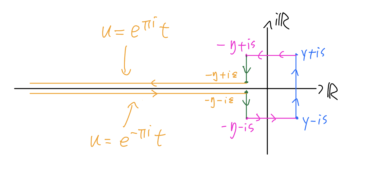
Observe that the integrand is bounded by
\[u^{1/2}\exp\left(2\pi\lambda_n^2u+{\pi\over12u}\right) \ll \begin{cases} e^{-2\pi n\varepsilon} & \Re(u)=-\varepsilon, \\ e^{2\pi ny} & \Re(u)\le y,\vert\Im(u)\vert=\frac12, \end{cases}\]When $\varepsilon,\eta\to0^+$, the integrals over the orange segments become
\[\begin{aligned} i^{-1}&\left(\int_{-\infty}^{-\eta-i\varepsilon}+\int_{-\eta+i\varepsilon}^{-\infty}\right) \\ &\to-2\int_0^\infty t^{1/2}\exp\left(-2\pi\lambda_n^2t+{\pi\over12t}\right)\mathrm dt:=-T(n) \end{aligned}\]Consequently, when
\[L(n)=i^{-1}\int_{-\infty}^{(0+)}u^{1/2}\exp\left(2\pi\lambda_n^2u+{\pi\over12u}\right)\mathrm du.\]we have
\[p^*(n)-[L(n)+T(n)]\ll e^{2\pi yn}\ll\exp\left(\frac\pi2\sqrt{n\over6}\right).\tag{16}\]Evaluation of $L(n)$
Using the Maclaurin series for $\exp(z)$, we have
\[L(n)=i^{-1}\sum_{v\ge0}{1\over v!}\left(\pi\over12\right)^v\int_{-\infty}^{(0+)}u^{\frac12-v}e^{2\pi\lambda_n^2u}\mathrm du.\]By Hankel's formula for the Gamma function, we have for $q>0$ that
\[{q^{z-1}\over\Gamma(z)}={1\over2\pi i}\int_{-\infty}^{(0+)} u^{-z}e^{q u}\mathrm du,\]so $L(n)$ becomes
\[\begin{aligned} L(n) &=\sum_{v\ge0}{2\pi\over v!\Gamma\left(v-\frac12\right)}\left(\pi\over12\right)^v(2\pi\lambda_n^2)^{v-\frac32} \\ &=(2\pi)^{-1/2}\lambda_n^{-3}G\left(\pi^2\lambda_n^2\over6\right), \end{aligned}\tag{17}\]where
\[G(X)=\sum_{v\ge0}{X^v\over v!\Gamma\left(v-\frac12\right)}.\]Because $\Gamma\left(\frac12\right)=\pi^{1/2}$, we have $\Gamma\left(-\frac12\right)=-2\pi^{1/2}$ and for $v\ge1$ that
\[\begin{aligned} v!\Gamma\left(v-\frac12\right) &=v!\Gamma\left(-\frac12\right)\left(-\frac12\right)\left(-\frac12+1\right)\cdots\left(-\frac12+v-1\right) \\ &=2^{-v}v!\Gamma\left(-\frac12\right)(-1)\times1\times3\times\cdots\times(2v-3) \\ &=4^{-v}(2v)!!\Gamma\left(-\frac12\right)(-1){(2v-1)!!\over2v-1} \\ &=2\pi^{1/2}{(2v)!!(2v-1)!!\over(2v-1)4^v}={2\pi^{1/2}(2v)!\over(2v-1)4^v}. \end{aligned}\]Consequently, when $Y^2=4X$, we have
\[\begin{aligned} G(X) &={1\over2\pi^{1/2}}\left[-1+\sum_{v\ge1}{(2v-1)Y^{2v}\over(2v)!}\right] \\ &={1\over2\pi^{1/2}}\left[-1+Y^2{\mathrm d\over\mathrm dY}\sum_{v\ge1}{Y^{2v-1}\over(2v)!}\right] \\ &={Y^2\over2\pi^{1/2}}{\mathrm d\over\mathrm dY}\left(\frac1Y\sum_{v\ge0}{Y^{2v}\over(2v)!}\right)={Y^2\over2\pi^{1/2}}{\mathrm d\over\mathrm dY}\left(\cosh Y\over Y\right). \end{aligned}\]For convenience, let $C=\pi\sqrt{2/3}$ and $X=\pi^2\lambda_n^2/6$, so we have $Y=C\lambda_n$ and
\[\begin{aligned} G(X) &={\lambda_n^2\over2\pi^{1/2}}{\mathrm d\over\mathrm d\lambda_n}\left(\cosh(C\lambda_n)\over\lambda_n\right) \\ &={\lambda_n^3\over\pi^{1/2}}{\mathrm d\over\mathrm dn}\left(\cosh(C\lambda_n)\over\lambda_n\right).\tag{18} \end{aligned}\]Plugging (18) into (17), we obtain
\[L(n)={1\over\pi\sqrt2}{\mathrm d\over\mathrm dn}\left(\cosh(C\lambda_n)\over\lambda_n\right).\tag{19}\]Evaluation of $T(n)$
Under the substitution $t=x^2$, we $\mathrm dt=2x\mathrm dx$
\[\begin{aligned} T(n) &=4\int_0^\infty x^2\exp\left(-2\pi\lambda_n^2x^2-{\pi\over12x}\right)\mathrm dx \\ &=-\frac2\pi{\mathrm d\over\mathrm d(\lambda_n^2)}\int_0^\infty\exp\left(-2\pi\lambda_n^2x^2-{\pi\over12x^2}\right)\mathrm dx.\tag{20} \end{aligned}\]For convenience, let $I(a,b)$ denote the integral
\[I(a,b)=\int_0^\infty e^{-a^2x^2-b^2x^{-2}}\mathrm dx.\]Under the change of variable $ax\mapsto b\rho^{-1}$, we have $\mathrm dx=-(b/a)\rho^{-2}\mathrm d\rho$
\[I(a,b)=\frac ba\int_0^\infty\rho^{-2}e^{-b^2\rho^{-2}-a^2\rho^2}\mathrm d\rho.\]This indicates that
\[\begin{aligned} 2a I(a,b) &=\int_0^\infty(a+bx^{-2})e^{-a^2x^2-b^2x^{-2}}\mathrm dx \\ &=e^{-2ab}\int_0^\infty e^{-(ax-bx^{-1})^2}\mathrm d(ax-bx^{-1}) \\ &=e^{-2ab}\int_{-\infty}^\infty e^{-\gamma^2}\mathrm d\gamma=\sqrt\pi e^{-2ab}, \\ \Rightarrow I(a,b)&={\sqrt\pi\over2a}e^{-2ab}. \end{aligned}\]When $a^2=2\pi\lambda_n^2$ and $b^2=\pi/12$, we have $2ab=C\lambda_n$, so (20) becomes
\[T(n)=-{1\over\pi\sqrt2}{\mathrm d\over\mathrm dn}\left({e^{-C\lambda_n}\over\lambda_n}\right).\]Hence, we have
\[L(n)+T(n)={1\over\pi\sqrt2}{\mathrm d\over\mathrm dn}\left(\sinh(C\lambda_n)\over\lambda_n\right).\]Combining this with (11) and (16) gives
\[p(n)={1\over\pi\sqrt2}{\mathrm d\over\mathrm dn}\left(\sinh(C\lambda_n)\over\lambda_n\right)+O(e^{\frac12C\sqrt n}).\tag{21}\]Because
\[\begin{aligned} {\mathrm d\over\mathrm dn}\left(e^{-C\lambda_n}\over\lambda_n\right) &={1\over2\lambda_n}{\mathrm d\over\mathrm d\lambda_n}\left(e^{-C\lambda_n}\over\lambda_n\right) \\ &={-C\lambda_n e^{-C\lambda_n}-e^{-C\lambda_n}\over2\lambda_n^3}\ll{e^{-C\lambda_n}\over\lambda_n^2}\ll e^{\frac12C\sqrt n}, \end{aligned}\]we find that replacing $\sinh(C\lambda_n)$ with $e^{C\lambda_n}/2$ in (21) produces the asymptotic formula (2). Plugging $n=200$ into the main term of (2), we have
\[p(200)\approx 3,972,998,993,186\]Compared with the true value $3,972,999,029,388$, this approximation has a relative error within $10^{-7}\%$ and an absolute error within $4\times10^4$, much better than the approximation (15) obtained by (1).
At $n=200$, (21) gives the same approximation as (2).
Conclusion
In this article, we presented two asymptotic formulas for $p(n)$ and gave a detailed account of their proofs. It should be noted that Hardy and Ramanujan1 did not obtain the function
\[\psi(n)={1\over2\pi\sqrt2}{\mathrm d\over\mathrm dn}\left(e^{C\lambda_n}\over\lambda_n\right)\]by computing the contour integral. Instead, they first defined the function and then analyze the error directly:
\[p(n)-a_n=\int_{\vert x\vert=r}\left(f(x)-\sum_{n\ge1}\psi(n)x^n\right){\mathrm dx\over x^{n+1}}.\]The Hankel integral approach in this article is adapted from Rademacher2. By analyzing the asymptotic behaviors of $f(x)$ near the roots of unities, Hardy and Ramanujan1 improved (2) to an asymptotic series:
\[p(n)={1\over2\pi\sqrt2}\sum_{k\le\alpha\sqrt{n}}A_k(n)k^{\frac12}{\mathrm d\over\mathrm dn}\left(e^{C\lambda_n}\over\lambda_n\right)+O(n^{-\frac14}),\tag{22}\]where $A_k(n)$ is a certain trigonometric sum. It is (22) that allows them to obtain the exact value of $p(200)$. As the proof of this asymptotic series invokes deep results from modular functions, we will not be discussing (22) until we have fully developed the theory.
-
Hardy, G. H., & Ramanujan, S. (1918). Asymptotic Formulae in Combinatory Analysis. Proceedings of the London Mathematical Society, s2-17(1), 75–115. ↩ ↩2
-
Rademacher, H. (1938). On the Partition Function $p(n)$. Proceedings of the London Mathematical Society, s2-43(1), 241–254. ↩