Cycloids and the tautochrone problem
special-functions real-analysisLet $c$ be a circle of radius $r>0$ centered at $(0,r)$ and label its intersection with origin by $P$. Now, we let $c$ roll on the $x$-axis without slipping. Then we can trace $P$ by the rotation angle $\theta$ of $c$.
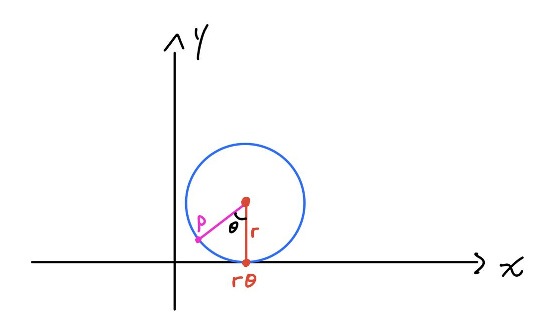
By some basic trigonometry, we find that $P=(x,y)$ fulfills the following relationship:
\[x=r(\theta-\sin\theta),\quad y=r(1-\cos\theta).\tag1\]The aggregate of $(x,y)$ obtained by varying $\theta$ from $0$ to $2\pi$ is known as cycloid curve:
By differentiating (1), we can easily compute the length of cycloid:
\[\mathrm dx=r(1-\cos\theta)\mathrm d\theta,\quad\mathrm dy=r\sin\theta.\] \[\begin{aligned} (\mathrm ds)^2 &=(\mathrm dx)^2+(\mathrm dy)^2=r^2[(1-\cos\theta)^2+\sin^2\theta](\mathrm d\theta)^2 \\ &=r^2(2-2\cos\theta)\mathrm d\theta^2=4r^2\sin^2\frac\theta2(\mathrm d\theta)^2. \end{aligned}\] \[\int_{\text{cycloid}}\mathrm ds=2r\int_0^{2\pi}\sin\frac\theta2\mathrm d\theta= 8r.\]Consequently, the length of a full cycloid is exactly 8 times the radius of its generating circle.
Cycloid is famous for solving the brachistochrone problem, which looks for curve connecting two points $A$ and $B$ such that $y_A>y_B$ and the time it takes for an object launched at rest at $A$ to reach $B$ is the minimal.
Since the brachistochrone problem is already standard exercise in calculus of variations and the solutions have been available all over the Internet, we decide to discuss a less well known problem in this article: the tautochrone problem.
In brief, the tautochrone problem seeks a curve $\gamma$ connecting two points $A$ and $B$ such that for any point $C$ on $\gamma$ excluding $B$, the time it takes for an object launching at $C$ to reach $B$ is constant.
The tautochrone problem
Assume $\gamma$ to be smooth and have length $L$. Let $\gamma(s):[0,L]\to\mathbb R^2$ be its arc length parametrization. Then $\gamma(0)=A$, $\gamma(L)=B$, and $\gamma(s_0)=C$ for some $0\le s_0<L$. The assumption that $\gamma$ is a tautochrone curve is equivalent to the claim that there exists some $T=T(A,B)>0$ such that
\[T=\int_\gamma\mathrm dt=\int_{s_0}^L{\mathrm ds\over(\mathrm ds/\mathrm dt)},\quad\forall 0\le s_0<L.\tag2\]To compute the velocity, we invoke the conservation of energy. Let $m$ be the mass of the object we launch, so
\[\frac12m\left(\mathrm ds\over\mathrm dt\right)^2+mgy=mgy_C\Rightarrow{\mathrm ds\over\mathrm dt}=\sqrt{2g(y_C-y)}.\]Plugging this into (2) gives
\[\sqrt{2g}T=\int_{y_C}^{y_B}(y_C-y)^{-\frac12}{\mathrm ds\over\mathrm dy}\mathrm dy.\]Let $f(u)$ denote ${\mathrm ds/\mathrm dy}$ evaluated at $y=y_B+u$ and $\tau=y_C-y_B>0$. Then the above expression is transformed into
\[-\sqrt{2g}T=\int_0^\tau(\tau-u)^{-\frac12}f(u)\mathrm du,\quad\forall 0<\tau\le \tau_0=y_A-y_B.\tag3\]The right hand side is a convolution of $\tau\mapsto\tau^{-\frac12}$ and $\tau\mapsto f(\tau)$, and a common way to demystify convolutions is through the use of Laplace transform.
Application of the Laplace transform
Let $Q$ denote the class of continuous function $\phi$ on $(0,+\infty)$ such that there exists $c=c(\phi)\in\mathbb R$ such that
\[\int_0^1\vert\phi(u)\vert\mathrm du<+\infty,\quad\forall u\ge1,\vert\phi(u)\vert\le e^{cu}.\tag4\]Then its Laplace transform $\mathcal L[\phi]$ is given by
\[\mathcal L[\phi]=\int_0^{+\infty}e^{-\tau\lambda}\phi(\tau)\mathrm d\tau.\]It is clear that $\mathcal L$ is a linear operator on $Q$.
Although we only require $f$ to be defined and satisfy (3) on $[0,\tau_0]$, the Laplace transform allows us to find a solution that satisfies (3) for all $\tau>0$.
On the right hand side of (3), computing the double integral gives1
\[\begin{aligned} \int_{\tau=0}^{+\infty}e^{-\tau\lambda} &\int_{u=0}^\tau(\tau-u)^{-\frac12}f(u)\mathrm du\mathrm d\tau \\ &=\int_{\tau=0}^{+\infty}\int_{u=0}^\tau e^{-(\tau-u)\lambda}(\tau-u)^{-\frac12}e^{-u\lambda}f(u)\mathrm du\mathrm d\tau \\ &=\int_{u=0}^{+\infty}e^{-u\lambda}f(u)\int_{\tau=u}^{+\infty}e^{-(\tau-u)\lambda}(\tau-u)^{-\frac12}\mathrm d\tau\mathrm du \\ &=\int_{u=0}^{+\infty}e^{-u\lambda}f(u)\int_{\alpha=0}^{+\infty}e^{-\alpha\lambda}\alpha^{-\frac12}\mathrm d\alpha\mathrm du \\ &=\mathcal L[f]\int_{\alpha=0}^{+\infty}e^{-\alpha\lambda}\alpha^{-\frac12}\mathrm d\alpha=\mathcal L[f]\mathcal L[\tau^{-\frac12}]. \end{aligned}\]For $\mathcal L[\tau^{-\frac12}]$, by substitution $\beta=\sqrt{\alpha\lambda}$, we have
\[\mathcal L[\tau^{-\frac12}]=2\lambda^{-\frac12}\int_0^{+\infty}e^{-\beta^2}\mathrm d\beta=\pi^{\frac12}\lambda^{-\frac12}.\]In addition, because $\mathcal L[1]=\lambda^{-1}$, we conclude that (3) becomes
\[-\sqrt{2g}T\lambda^{-1}=\mathcal L[f]\pi^{\frac12}\lambda^{-\frac12},\]so solving for $\mathcal L[f]$ gives
\[\mathcal L[f]=-{\sqrt{2g}T\over\pi}\pi^{\frac12}\lambda^{-\frac12}=\mathcal L\left[-{\sqrt{2g}T\over\pi}\tau^{-\frac12}\right].\tag5\]From (5), we can conclude that
\[f(\tau)=-{\sqrt{2g}T\over\pi}\tau^{-\frac12}.\tag6\]is a solution to (3). By plugging in the definition of $f$ and $\tau$, we have the following
\[{\mathrm ds\over\mathrm dy}=-{\sqrt{2g}T\over\pi}(y_B-y)^{-\frac12}.\tag7\]This gives the arc length parametrization of the tautochrone curve. To extract more information, we need to find a better parametrization.
Parametric equation of the tautochrone curve
Let $\mathrm dy/\mathrm dx=\tan\theta$. Then we have $({\mathrm ds/\mathrm dy})^2=1+(\mathrm dx/\mathrm dy)^2=\csc^2\theta$, so (7) becomes
\[y={2gT^2\over\pi^2}\sin^2\theta+y_B={gT^2\over\pi^2}(1-\cos2\theta)+y_B\tag8.\]This indicates that $\theta_B=0$. To obtain the equation of $x$, notice that
\[{\mathrm dx\over\mathrm d\theta}={\mathrm dx\over\mathrm dy}\cdot{\mathrm dy\over\mathrm d\theta}=\cot\theta{4gT^2\over\pi^2}\sin\theta\cos\theta={4gT^2\over\pi^2}\cos^2\theta.\]Integrating and equating the value at $\theta=\theta_B$, we deduce
\[x={gT^2\over\pi^2}(2\theta+\sin2\theta)+x_B.\tag9\]Let $\phi=2\theta+\pi$. Then (8) and (9) become
\[\begin{cases} \displaystyle x={gT^2\over\pi^2}(\phi-\sin\phi)+x_B-{gT^2\over\pi^2}, \\ \displaystyle y=-{gT^2\over\pi^2}(1-\cos\phi)+y_B+{2gT^2\over\pi^2}. \end{cases}\tag{10}\]From our analysis of (8), $\phi_B=\pi$. Solving (10) at $(x,y)=(x_A,y_A)$ gives $T$ and $\phi_A$. Therefore, comparing to (1), we conclude that a solution to the tautochrone problem is given by the inverted cycloid of radius $gT^2/\pi^2$.
For the sake of completeness, we give a rigorous proof that there are no solutions to the tautochrone problem other than cycloids.
Uniqueness of the solution
Since the parametric equations (10) are derived from the expression $f(\tau)$, it suffices to show that (3) has a unique solution.
Let $\phi$ be a continuous function on $(0,\tau_0]$ and absolutely integrable (in the improper sense) on $[0,\tau_0]$. Then for all $0<\tau\le\tau_0$, the integral2
\[I_\alpha[\phi](\tau)={1\over\Gamma(\alpha)}\int_0^\tau(\tau-u)^{\alpha-1}\phi(u)\mathrm du\tag{11}\]converges absolutely and defines an analytic function of $\alpha$ in $\Re\alpha>0$. Notice that
\[\begin{aligned} (I_\alpha\circ I_\beta)[\phi](\tau) &={1\over\Gamma(\alpha)\Gamma(\beta)}\int_{t=0}^\tau(\tau-t)^{\alpha-1}\int_{u=0}^t(t-u)^{\beta-1}\phi(u)\mathrm du\mathrm dt \\ &={1\over\Gamma(\alpha)\Gamma(\beta)}\int_{u=0}^\tau\phi(u)\underbrace{\int_{t=u}^\tau(\tau-t)^{\alpha-1}(t-u)^{\beta-1}\mathrm dt}_{t=(\tau-u)v+u}\mathrm du \\ &={1\over\Gamma(\alpha)\Gamma(\beta)}\int_{u=0}^\tau\phi(u)\underbrace{\int_0^1(1-v)^{\alpha-1}v^{\beta-1}\mathrm dv}_{\Gamma(\alpha)\Gamma(\beta)/\Gamma(\alpha+\beta)}(\tau-u)^{\alpha+\beta-1}\mathrm du \\ &={1\over\Gamma(\alpha+\beta)}\int_{u=0}^\tau(\tau-u)^{\alpha+\beta-1}\phi(u)\mathrm du, \end{aligned}\]so we have
\[(I_\alpha\circ I_\beta)[\phi](\tau)=I_{\alpha+\beta}[\phi](\tau).\tag{12}\]This reasonably poses the question that whether $\phi$ can be obtained from (12) by making $\beta\to-\alpha$.
Lemma 1: If $\phi$ is absolutely integrable on $[0,\tau_0]$ and continuous at $\tau\in(0,\tau_0]$, then
\[\lim_{\alpha\to0^+}I_\alpha[\phi](\tau)=\phi(\tau).\]Proof. When $\alpha\to0^+$, it is obvious that
\[\lim_{\alpha\to0^+}\phi(\tau)I_\alpha[1](\tau)=\lim_{\alpha\to0^+}{\tau^\alpha\phi(\tau)\over\Gamma(\alpha+1)}=\phi(\tau),\]so it suffices to show that
\[\lim_{\alpha\to0^+}\underbrace{I_\alpha[\phi](\tau)-\phi(\tau)I_\alpha[1](\tau)}_{\Delta_\alpha}=0.\]By continuity, there exists some $\delta>0$ such that $\vert\phi(u)-\phi(\tau)\vert$ for $\tau-\delta<u\le\tau$, so when $0<\alpha<1$, there is
\[\begin{aligned} \vert\Delta_\alpha\vert &<{\varepsilon\over\Gamma(\alpha)}\int_{\tau-\delta}^\tau(\tau-u)^{\alpha}\mathrm du+{1\over\Gamma(\alpha)}\int_0^{\tau-\delta}(\tau-u)^{\alpha-1}\vert\phi(u)-\phi(\tau)\vert\mathrm du \\ &\le {\varepsilon\delta^\alpha\over\Gamma(\alpha+1)}+{\delta^{\alpha-1}\over\Gamma(\alpha)}\int_0^\tau[\vert\phi(u)\vert+\vert\phi(\tau)\vert]\mathrm du. \end{aligned}\]This indicates that $\limsup_{\alpha\to0^+}\vert\Delta_\alpha\vert\le\varepsilon$ for all $\varepsilon>0$. $\square$
Lemma 2: $I_\alpha[\phi]$ is injective over all $\phi$ continuous on $(0,\tau_0]$ and absolutely integrable on $[0,\tau_0]$.
Proof. Since $I_\alpha$ is a linear operator, it suffices to show that if $\phi$ is continuous on $(0,\tau_0]$ and integrable on $[0,\tau_0]$, then for any $\alpha>0$, if
\[I_\alpha[\phi](\tau)\equiv0,\quad\forall 0<\tau\le\tau_0,\tag{13}\]then $\phi(\tau)\equiv0$. Plugging (13) into (12), we have
\[I_{\alpha+\beta}[\phi](\tau)\equiv0,\quad\forall 0<\tau\le\tau_0\]for all $\beta>0$. By analytic continuation, this is valid for all $\beta>-\alpha$. Therefore, by Lemma 1, for any $0<\tau\le\tau_0$, there is
\[\phi(\tau)=\lim_{\beta\to-\alpha^+}I_{\alpha+\beta}[\phi](\tau)=0,\]so $\phi$ is identically zero. $\square$
Observe that (3) can be written as
\[-{\sqrt{2g}T\over\Gamma(\frac12)}=I_{\frac12}[f](\tau),\quad\forall 0<\tau\le\tau_0,\]so by Lemma 2, we conclude that
Uniqueness theorem: If $f$ is continuous on $(0,\tau_0]$, absolutely integrable on $[0,\tau_0]$, and satisfies (3), then (6) is the only admissible $f$.
From the physicists' point of view, everything is assumed to be smooth, so this theorem guarantees that cycloids are the only class of smooth curve that solves the tautochrone problem.
Conclusion
In this article, we began our discussion by constructing the cycloid by rolling a circle. After investigating its basic geometric properties, we turned our attention to the tautochrone problem. Following an invocation of the Laplace transform, we showed that the cycloid curve is a solution to the problem. Finally, by examining the behaviors of the $I_\alpha$ operators, we prove that cycloid is the only smooth solution of the tautochrone problem.
In essence, our investigation demonstrates an intrinsic relationship between physics and pure mathematics.
-
This is a special case of the convolution theorem. ↩
-
This is known as the Riemann-Liouville integral. ↩